Delta-Rule and Online Learning

Opening: the Unification Quadruple

Before the operator-by-operator derivation in the rest of the chapter, it is worth pausing on a striking observation: GLA, Mamba-2, RetNet, mLSTM, and DeltaNet are all the same underlying operator viewed through four different lenses. Four anchor papers each derive this unification from a different starting point, and the four derivations converge on the same family. We call the collection the Unification Quadruple; once any one lens is internalized the others become re-derivations rather than new content.

The pedagogical payoff for Week 12 is concrete. The implicit-versus-explicit numerical-integration pair — which is the load-bearing content of the DeltaNet and Longhorn sections below — lives most naturally under the Longhorn lens. Sequencing Longhorn → UIA → FWP → SSD lets the reader anchor on the ODE intuition first, then watch the same object reappear as an implicit-attention computation, then as a fast-weight programmer, then as a structured-matrix product. Each subsequent lens reuses the same moving parts.

Lens 1 — Longhorn: amortized online learning

The Longhorn paper Liu et al. (2024) (ICLR 2025) reformulates the SSM recurrence as the closed-form solution to a per-token online learning objective:

a Tikhonov-regularised retrieval problem with closed form $\bm{S}_t = (\alpha\bm{S}_{t-1} + \bm{v}_t\bm{k}_t^\top)(\alpha\bm{I} + \bm{k}_t\bm{k}_t^\top)^{-1}$. The DeltaNet update is the first-order explicit step of gradient descent on the same per-token loss; the Longhorn update is the closed-form implicit step on the regularised version. In ODE language: DeltaNet is forward Euler on the per-token learning ODE; Longhorn is the implicit midpoint / backward-Euler companion. Their stability regions differ accordingly, and so do their effective learning rates (Longhorn’s $\beta_\text{eff}=1/(\alpha+\norm{\bm{k}}^2)$ is automatically bounded; DeltaNet’s $\beta_t$ must be clipped to remain conditionally stable).

Lens 2 — UIA: unified implicit attention

The Unified Implicit Attention paper Anonymous (2024) (ICLR 2025) proves that gated linear RNNs — Mamba, RWKV, GLA — implement the same implicit-attention computation despite their different surface parameterisations. The argument shows that each architecture’s recurrence rolls out into a fixed-rank dot-product attention with a particular gating schedule; differences between architectures collapse into different choices of which function maps the input to the attention pattern, not into different operators. Under this lens the DeltaNet update reads as one step of implicit attention with a rank-one correction — exactly the “selective erasure then write” interpretation we will use throughout the DeltaNet section.

Lens 3 — FWP: fast weight programming

The fast-weight programming survey Anonymous (2025) (2025) frames GLA, Mamba-2, RetNet, mLSTM, and DeltaNet as instances of Schmidhuber’s 1992 fast-weight programmers: the recurrent state is a learned weight matrix that the model updates online, and the architecture’s choice of update rule is the choice of programmer. DeltaNet’s update — erase by an outer product, then write a new outer product — is the canonical FWP rule. The lens is useful because it makes the per-token capacity of the state explicit: matrix-valued state $\bm{S}_t \in \R^{d_v \times d_k}$ stores exactly $d_v \cdot d_k$ scalar parameters, regardless of how the update rule is written.

Lens 4 — SSD: structured state-space duality

Structured State-Space Duality Dao & Gu (2024) Anonymous (2025) proves that a scalar-state SSM is exactly an attention computation with a 1-semiseparable lower-triangular mask. The state-space view and the attention view are formally equivalent under this restriction; the two computations differ only in the algorithmic order in which the matrix product is evaluated. Mamba-2 ([?ch:week08]) is the engineered realisation of the attention-order traversal; the recurrence view is the SSM-order traversal of the same underlying object. Once SSD is internalised, the DeltaNet recurrence and a masked-attention forward pass are different schedulings of one algorithm.

The delta rule as online learning

DeltaNet Yang et al. (2024) stores a fast-weight matrix $\bm{S}_t \in \R^{d_v \times d_k}$ as recurrent state, updated each step from a key/value/learning-rate triple $(\bm{k}_t, \bm{v}_t, \beta_t)$. The recurrence is

The first factor $(\bm{I} - \beta_t \bm{k}_t \bm{k}_t^\top)$ performs selective erasure along the $\bm{k}_t$ direction; the second adds the new association as a rank-one outer product. Materialising the $d_k \times d_k$ erase factor is wasteful: the textbook delta-rule rearrangement

uses one matrix-vector product (cost $\bigO{d_v d_k}$) and one rank-one update (cost $\bigO{d_v d_k}$) per step — the same big-$O$ as Mamba’s diagonal scan from Week 7. The reference implementation is in delta_rule.py :delta_rule_step; the rank-one form is the only path used at runtime, with the explicit erase form retained only as a Python-loop oracle in delta_rule_naive for test coverage. [Practitioner]

Reading the recurrence as gradient descent

The rank-one form is, line for line, one step of explicit gradient descent on the per-token retrieval-error objective

The gradient with respect to $\bm{S}$ is the rank-one matrix $(\bm{S}\bm{k}_t - \bm{v}_t)\bm{k}_t^\top$, and one gradient step with step size $\beta_t$ gives exactly the DeltaNet recurrence. So DeltaNet is literally an online learner whose “parameter vector” is its recurrent state and whose per-step loss is the squared error of retrieving $\bm{v}_t$ at $\bm{k}_t$. [Official]

Longhorn: the implicit step

If DeltaNet is one explicit gradient step on the retrieval-error loss, Longhorn Liu et al. (2024) performs the closed-form solve of a Tikhonov-regularised version of the same objective:

The first term is the per-token retrieval loss; the second is a quadratic penalty that keeps $\bm{S}_t$ close to $\bm{S}_{t-1}$. The weight $\alpha_t > 0$ is a trust-region parameter — large $\alpha_t$ keeps the state mostly unchanged, small $\alpha_t$ allows aggressive fitting.

Setting the gradient with respect to $\bm{S}$ to zero gives the implicit recurrence

The implicit reference to $\bm{S}_t$ on both sides looks problematic at first glance, but the structure is rank-one and admits a closed-form solution. Right-multiply both sides by $\bm{k}_t$ to isolate $\bm{S}_t \bm{k}_t$, then substitute back to recover:

So Longhorn looks structurally identical to DeltaNet, but with an effective learning rate

The denominator is exactly what makes the step implicit: it self-adapts to the magnitude of $\bm{k}_t$ so that the effective rate stays in $\bigl(0,\, 1/\alpha_t\bigr]$ no matter how large $\bm{k}_t$ gets. The reference implementation is longhorn.py :longhorn_step; the calibrated-rate equivalence to DeltaNet is asserted in test_longhorn.py:test_longhorn_matches_deltanet_at_calibrated_rate. [Official]

Stability regions: explicit vs implicit

Let $\bm{S}^\star = \bm{v}\bm{k}^\top / \norm{\bm{k}}^2$ be the unique fixed point of either iteration when keys and values are held constant at $(\bm{k}, \bm{v})$. (This is the rank-one state that retrieves $\bm{v}$ at $\bm{k}$.) Linearising the iteration around the fixed point and writing $\bm{E}_t = \bm{S}_t - \bm{S}^\star$, both algorithms reduce to the rank-one contraction

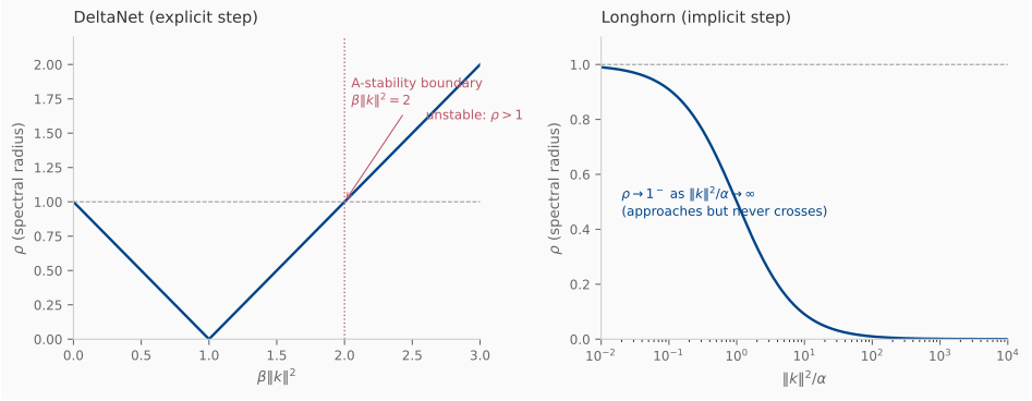
The eigenvalues of $(\bm{I} - \beta_{\text{eff}} \bm{k}\bm{k}^\top)$ are: one along $\bm{k}$ with value $1 - \beta_{\text{eff}} \norm{\bm{k}}^2$, and $d_k - 1$ along directions orthogonal to $\bm{k}$ with value $1$. The orthogonal-direction eigenvalues equal one because neither algorithm corrects deviations in directions it has not seen a key for; that is the persistent-memory feature of fast-weights, not a stability concern. What matters for the along-$\bm{k}$ stability is the spectral radius

The two algorithms pick $\beta_{\text{eff}}$ differently: DeltaNet uses the unconstrained learnable rate $\beta_{\text{eff}} = \beta_t$; Longhorn uses the implicit rate $1/(\alpha_t + \norm{\bm{k}_t}^2)$.

The DeltaNet A-stability boundary

Past the boundary, $\rho_k > 1$ and the deviation alternates sign while its magnitude grows geometrically — exactly the explicit-Euler instability mode. [Convergence]

Longhorn unconditional stability

So Longhorn’s effective $\beta_{\text{eff}} \norm{\bm{k}}^2 = \norm{\bm{k}}^2 / (\alpha + \norm{\bm{k}}^2) < 1$ stays well inside the DeltaNet stability region. [Official]

Numerical validation

The analytic spectral-radius formulas are exposed as named functions in stability_analysis.py . The test file test_stability_analysis.py (26 tests) cross-checks each formula against the actual eigenvalue of the iteration matrix $(\bm{I} - \beta_{\text{eff}} \bm{k}\bm{k}^\top)$ computed numerically via Rayleigh quotient. If any formula drifts from the operator definition — for example, a sign error introduced when refactoring delta_rule.py — the test asserting $|\text{numerical}| = |\text{analytic}|$ catches it. [Practitioner]

Chunkwise factorization and the WY representation

The recurrent driver in delta_rule.py :delta_rule_recurrent is $\bigO{L}$ sequential. To match a transformer’s hardware throughput, DeltaNet’s chunkwise formulation Yang et al. (2024) exposes within-chunk parallelism. Split the length-$L$ sequence into chunks of size $C$. For chunk $c$ covering steps $t \in \{c_0, \ldots, c_0 + C - 1\}$ the recurrence unrolls to

where the chunk’s erase product is

and the chunk write contribution $\bm{R}_c$ is the suffix-product-weighted sum of the per-step rank-one writes. So the cross-chunk recurrence reduces to one rank-$d_k$ update per chunk: $\bigO{L/C}$ steps instead of $\bigO{L}$.

The Householder/WY identity

The chunk erase product $\bm{P}_c$ admits the Householder/WY representation

where $\bm{W}_c, \bm{Y}_c \in \R^{C \times d_k}$ are built recursively. Setting $\bm{Y}_c$ to the chunk’s keys (one row per step), the running-product recursion gives the new $\bm{W}_c$ row

which is the in-chunk equivalent of running the DeltaNet recurrence on $(\bm{k}_t, \beta_t)$ alone — a recipe directly analogous to the QR-factorisation Householder accumulator. [Convergence]

The proof is by induction on the chunk length: each factor $(\bm{I} - \beta_t \bm{k}_t \bm{k}_t^\top)$ contributes one new row to $\bm{W}_c$ and one to $\bm{Y}_c$, expanding $\bm{I} - \bm{W}_{c, \le t}^\top \bm{Y}_{c, \le t}$ into the next factor of the running product. The reference implementation is in chunkwise.py :chunk_wy_representation; the equivalence to the explicit erase product is asserted in test_chunkwise.py:test_wy_product_matches_explicit_erase_product across random seeds and chunk sizes 1 through 8.

Once $(\bm{W}_c, \bm{Y}_c)$ is available, applying $\bm{P}_c$ to the state matrix is one $(d_v \times C) + (C \times d_k)$ pair of GEMMs rather than $C$ rank-one updates:

This is the matmul-friendly form that production fused kernels exploit. The reference is chunkwise.py:apply_wy_to_state.

Chunkwise driver in pure JAX

The driver in chunkwise.py:delta_rule_chunkwise is a Python for loop over chunks. Each chunk is processed by a jax.lax.scan that takes the running state as its initial carry and emits the per-step outputs $\bm{o}_t = \bm{S}_t \bm{q}_t$. This implementation is intentionally pedagogical: real production gains require fused kernels we do not have in pure JAX (the within-chunk read in fused implementations runs in parallel via the WY identity). The WY primitives are exposed in-tree nonetheless so a future fused-kernel rewrite has a tested reference. [Practitioner]

The chunkwise-vs-recurrent equivalence is asserted in test_chunkwise.py:test_chunkwise_matches_recurrent for chunk sizes 1, 2, 4, 8, 16 (every divisor of the test sequence length 16). The unit tests double as a debugging surface: any future edit to the chunkwise decomposition or WY identity that breaks an identity will be flagged before merge.

What Week 12 buys you

1. An online-learning lens on linear attention. The retrieval-error loss reframes “fast-weight rule” as “per-token gradient step”, collapsing DeltaNet, Longhorn, and Gated DeltaNet into one family parameterised by the rate $\beta_t^{\text{eff}}$. The same lens transfers to Kimi Linear’s KDA Team (2025) and beyond.

2. A first-principles stability story. The spectral-radius analysis is the forward-Euler/implicit-midpoint pair from numerical integration applied to a neural recurrence. The DeltaNet A-stability boundary $\beta\norm{\bm{k}}^2 = 2$ and Longhorn’s unconditional stability are not empirical observations; they are theorems derivable from the rank-one structure alone.

3. A chunkwise refactor with a tested WY identity. The chunkwise decomposition reduces the $\bigO{L}$ cross-chunk recurrence to $\bigO{L/C}$, and the WY identity turns each chunk’s erase product into one matmul. The reference primitives in chunkwise.py are written so a future fused-kernel pass has a checked entry point rather than a fresh derivation.

4. The bridge to Weeks 13–14. Gated DeltaNet (W13) extends the trust-region weight $\alpha_t$ from a scalar to a data-dependent operator; the spectral-radius analysis here parameterises the result. The within-chunk parallel variant (W14) replaces the chunkwise scan with the WY-based block algorithm whose primitives are already exposed.

The implementation reference for the entire chapter is . Run pytest experiments/jax/week12/ to validate every claim: 75+ tests cover recurrent-vs-naive equivalence, calibrated-rate equivalence between Longhorn and DeltaNet, analytic-vs-numerical spectral radii, the WY identity, and chunkwise-vs-recurrent equivalence across all divisor chunk sizes.