S4 / HiPPO: Continuous to Discrete
Implement S4 from continuous-time SSM through HiPPO initialization, ZOH/bilinear discretization, and the recurrent/convolutional duality that makes S4 practical. The pedagogical bridge that underpins every selective SSM in production.
On this page
- The continuous SSM
- HiPPO: principled initialization
- Discretization: continuous to discrete
- Zero-Order Hold (ZOH)
- Bilinear (Tustin) transform
- Three views of SSM computation
- Recurrent view
- Convolutional view
- Mode switching
- The S4 layer in Flax NNX
- Post-training eigenvalue analysis
- Reflections
- What transfers
- What requires adaptation
- Forward map
The continuous SSM
The starting point is the state-space representation — a standard way to describe dynamical systems in control theory and signal processing. Any system of linear ordinary differential equations (ODEs) can be written in this form: The SSM deep learning literature adopted this formulation from the HiPPO paper Gu et al. (2020) .
where is the hidden state (a vector that summarizes the system’s memory — not to be confused with “state” in the ML training sense), is the scalar input, is the scalar output, and the system is defined by four matrices: (dynamics — how the state evolves), (how input enters the state), (how state maps to output), and (direct input-to-output skip connection). These matrices are time-invariant: the same values apply at every time step. This is the Linear Time-Invariant (LTI) assumption that makes the convolutional view possible (later section). Mamba (Week 7) breaks LTI by making , , input-dependent, gaining content-based selection but losing the convolutional view.
The connection to Week 1 is direct: the damped oscillator is exactly the continuous SSM with and . Now will be learned, not hand-crafted — but the stability requirements are identical: eigenvalues in the left half-plane.
HiPPO: principled initialization
The central question is: how do we initialize ? Random initialization leads to vanishing or exploding dynamics — the same pathology that makes recurrent neural networks difficult to train.
HiPPO (High-order Polynomial Projection Operators) Gu et al. (2020) provides a principled answer: initialize so that the state encodes the best -term Legendre polynomial approximation of the input history for . Legendre polynomials are an orthogonal basis for representing functions on an interval — the optimal choice for approximating smooth signals with a finite number of coefficients. The state vector’s -th entry holds the -th Legendre coefficient of the input history, giving the SSM a mathematically principled “memory” of the past.
The HiPPO-LegS (Legendre, Scaled) matrix is:
The input matrix is .
The small-dimensional structure fits on one line of paper:
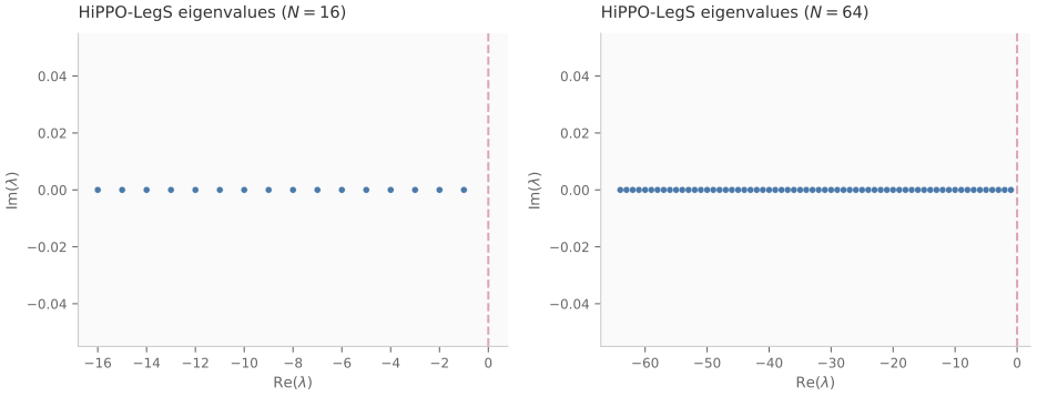
is lower-triangular with diagonal , so those are exactly the eigenvalues (each strictly negative). is a similarity transform, so inherits the same spectrum. For arbitrary the pattern continues: eigenvalues , stability guaranteed by construction.
All eigenvalues of have strictly negative real part: for all . For the local LegS construction used in this guide, they are exactly up to floating-point roundoff.
The similarity transform preserves eigenvalues. The matrix is lower-triangular with diagonal entries , so its eigenvalues are exactly . The same therefore holds for , placing the entire spectrum in the open left half-plane. Strict negativity is also checked numerically for in the week 4 test test_hippo_eigenvalues_negative_real.
Discretization: continuous to discrete
Discretization here means converting a continuous-time ODE (, defined for all ) into a discrete-time recurrence (, defined at integer time steps). This is the same process as converting a differential equation into a difference equation for numerical simulation — but here the step size is a learnable parameter, not a fixed choice. Note: “discretization” in NLP often means tokenization; here it strictly means ODE-to-recurrence conversion.
Given , we seek discrete matrices such that:
Zero-Order Hold (ZOH)
Zero-Order Hold (ZOH) assumes the input is piecewise constant over each discretization interval — that is, the input doesn’t change between time steps. This is a reasonable assumption when the step size is small relative to the input’s rate of change, which is the typical regime for SSMs. ZOH is the default discretization across S4, S4D, S5, and Mamba reference implementations. [Convergence] The resulting formulas are:
We avoid computing by using the stacked matrix exponential: build the augmented matrix , compute its expm, and extract , from the result. Implemented in s4_hippo.py:discretize_zoh .
This works because the block matrix exponential satisfies
so a single expm call yields both (top-left block) and (top-right block) without explicitly inverting .
If and , then .
since and .
Bilinear (Tustin) transform
The bilinear transform maps the imaginary axis to the unit circle:
This is second-order accurate, vs. first-order for forward Euler.
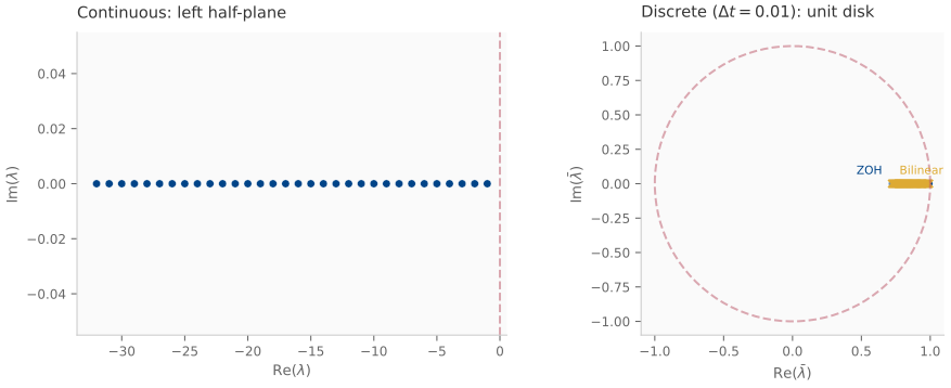
If all eigenvalues of lie in the open left half-plane () and , then all eigenvalues of lie strictly inside the unit disk ().
The bilinear transform maps eigenvalue of to eigenvalue of via the Möbius map (a fractional linear transformation of the complex plane):
Write with . Then and . Since , we have , giving and therefore . Geometrically, the bilinear transform maps the left half-plane exactly to the open unit disk — it is the standard conformal map (an angle-preserving holomorphic bijection) between these two stability regions.
Three views of SSM computation
An LTI SSM can be computed in two equivalent ways, enabling the train-fast / infer-cheap trick that makes S4 practical.
Recurrent view
The discrete state update is a direct recurrence computed via lax.scan with sequential steps and memory per token. This is the same scan primitive from Week 1, with and .
Convolutional view
The term “kernel” here means a convolution filter — a fixed sequence of coefficients that defines a weighted combination of nearby inputs. This is the signal processing sense, unrelated to kernel methods in classical ML (support vector machines, Gaussian processes) or operating system kernels.
Expanding the recurrence with gives:
where is the SSM kernel. This is a causal convolution (output at time depends only on inputs at times ), computed in via FFT.
Our implementation computes via iterative matrix powers in a lax.scan — , deliberately naive. Production S4 exploits DPLR (Diagonal Plus Low-Rank) structure to evaluate via Cauchy matrices (matrices with entries , enabling fast structured products) in .
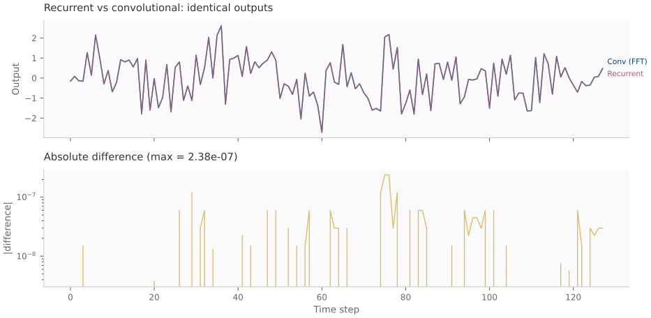
For an LTI SSM with , the recurrent scan and causal FFT convolution produce identical outputs.
By induction. The recurrence gives . Left-multiplying by yields the Toeplitz convolution with kernel . FFT computes exactly this (with zero-padding to avoid circular artifacts). Verified numerically at in the week 4 test test_recurrent_convolutional_equivalence.
Mode switching
S4’s practical trick: convolutional mode for training ( parallel) and recurrent mode for inference ( per token). Both modes share the same parameters; only the computation changes.
The S4 layer in Flax NNX
The S4Layer module wraps the SSM as a Flax NNX module, with parameters split by type for dual-optimizer treatment:
- SSMParam: , , — SSM optimizer (Adam, LR , no weight decay)
- nnx.Param: , , encoder, decoder — backbone optimizer (AdamW, LR , WD )
This is the same SSMParam split from Week 2. The week 2 harness works unchanged: the dual optimizer filters SSMParam variables with wrt=SSMParam.
class S4Layer(nnx.Module):
    def __init__(self, d_state=32, *, rngs):
        A, B = make_hippo_legs(d_state)
        self.A = SSMParam(A)
        self.B = SSMParam(B.squeeze())
        self.C = nnx.Param(random.normal(rngs.params(), (d_state,)))
        self.D = nnx.Param(jnp.ones(()))
        self.log_dt = SSMParam(...)  # log-uniform in [log(0.001), log(0.1)]
The S4SeqModel is a drop-in for SimpleSeqModel (Week 2), preserving the contract. With features and , the S4SeqModel has ~35K parameters vs. ~2K for SimpleSeqModel.
Post-training eigenvalue analysis
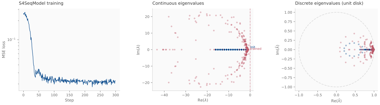
After training, we extract the learned matrices and verify stability:
- Continuous: (left half-plane)
- Discrete: (inside unit disk)
The low learning rate on SSMParam keeps eigenvalue drift small.
[Official]
The two-LR recipe (Adam on SSM params, AdamW on backbone) originates in the S4 paper Gu et al. (2020)
and reproduces across S4D, S5, and Mamba reference code.
Week 18 performs full Lyapunov stability analysis of trained SSMs, using the QR-based infrastructure from Week 1.
Reflections
What transfers
- Discretization awareness: The choice of integrator (Euler, ZOH, bilinear) determines training stability — exactly as in numerical PDE solvers.
- Eigenvalue monitoring: Checking after training is the SSM equivalent of checking CFL conditions.
- Dual computation modes: The recurrent/convolutional duality is unique to LTI systems and is lost in selective models (Week 7+).
What requires adaptation
- is learned, not given. In your PhD, the state matrix comes from physics. In S4, HiPPO provides a principled initialization, but training moves — possibly off the stability manifold. This is why the ZOH stability proposition only bounds initialization; post-training stability is a Week 18 question.
- Diagonalization is not free. Week 5’s S4D simplification abandons the HiPPO theoretical interpretation. The diagonal form reproduces S4’s empirical performance but loses the Legendre-polynomial memory interpretation — a theory-for-speed trade-off with no clean analogue in numerical PDE solvers.
Forward map
- Week 5: S4D makes diagonal, collapsing the kernel to .
- Week 6: S5 replaces
lax.scanwith associative scan for parallel depth. - Week 7: Mamba makes input-dependent, breaking the convolutional view.
- Week 18: Lyapunov analysis of trained S4 layers using Week 1 QR infrastructure.
- Week 9 (Julia): ZOH, bilinear, and exponential-trapezoidal compared on a forced oscillator, with empirical order-of-accuracy verification in
experiments/julia/week09/discretization.jl. - Week 20: Stability regions plotted as contour heatmaps in the complex plane,
experiments/julia/week20/stability_regions.jl.