Flax NNX Modules and Training Loop
Build the minimal training pipeline reused for every SSM experiment in the curriculum: NNX modules, dual-optimizer pattern, nnx.scan for layer stacking, and the SSMParam variable type.
On this page
From Linen to NNX
Flax is JAX’s primary neural network library (analogous to PyTorch’s nn module). Flax NNX (Neural Network eXperimental) is the current API as of Flax 0.12 (March 2026). The previous API, called Linen, used a functional style where parameters lived outside the module; NNX uses a more familiar object-oriented style where parameters are Python attributes. All code in this curriculum uses NNX.
| Aspect | Linen (legacy) | NNX (current) |
|---|---|---|
| Initialization | Lazy setup() | Eager __init__ |
| Parameters | self.param('name', init, shape) | Normal Python attributes |
| Mutable state | self.variable('cache', ...) | nnx.Variable(...) attribute |
| Scan layers | nn.scan(Module, ...) | nnx.vmap plus nnx.scan |
| Train state | TrainState | nnx.Optimizer |
mamba2-jax reference repo in experiments/refs/ already uses NNX — it serves as our style guide for SSM modules.
The most important change for training: nnx.Optimizer requires a wrt= (“with respect to”) argument specifying which variable type to optimize. For example, wrt=SSMParam means “only update variables of type SSMParam; ignore all others.” This enables the dual-optimizer pattern central to SSM training: one optimizer for the SSM’s internal parameters (, , ) at a lower learning rate, and a separate optimizer for the rest of the network at a higher learning rate.
[Official]
Originally recommended in the S4 paper Gu et al. (2020)
; reproduced across S4D, S5, and Mamba reference code.
The sequence model as module
A minimal Conv1D → MLP sequence model demonstrates the NNX module pattern:
class SimpleSeqModel(nnx.Module):
    def __init__(self, features, kernel_size=3, *, rngs):
        self.conv = nnx.Conv(1, features, kernel_size, rngs=rngs)
        self.dense1 = nnx.Linear(features, features, rngs=rngs)
        self.dense2 = nnx.Linear(features, 1, rngs=rngs)

    def __call__(self, x):  # (B, L, 1) -> (B, L, 1)
        h = nnx.relu(self.conv(x))
        h = nnx.relu(self.dense1(h))
return self.dense2(h)For input tensor , SimpleSeqModel returns . SAME padding keeps the sequence length unchanged, matching Flax’s default Conv1D behavior.
Conv1D: with SAME padding. Dense1: . Dense2: . Sequence length is preserved at every stage.
The training loop
The NNX training pattern differs fundamentally from PyTorch. In PyTorch, you call separate functions for zeroing gradients, running the forward pass, computing gradients (backpropagation), and updating parameters. In JAX, these are composed into a single function that is compiled and executed as one unit:
| Step | PyTorch | JAX/NNX |
|---|---|---|
| Zero gradients | optimizer.zero_grad() | (not needed) |
| Forward pass | y = model(x) | nnx.value_and_grad(loss_fn) |
| Backward pass | loss.backward() | returns loss and gradients together |
| Update params | optimizer.step() | optimizer.update(model, grads) |
| Compile | torch.compile(model) | @nnx.jit (wraps entire step) |
value_and_grad: returns loss and gradients together; JAX traces once into XLA and runs forward+backward as one graph.
@nnx.jit
def train_step(model, optimizer, x, y):
    def loss_fn(model):
        return jnp.mean((model(x) - y) ** 2)
    loss, grads = nnx.value_and_grad(loss_fn)(model)
    optimizer.update(model, grads)  # in-place
return lossoptimizer.update() requires both model and grads as arguments (changed from single-argument in earlier versions). The wrt= filter on the optimizer handles extracting the relevant subset of gradients internally.
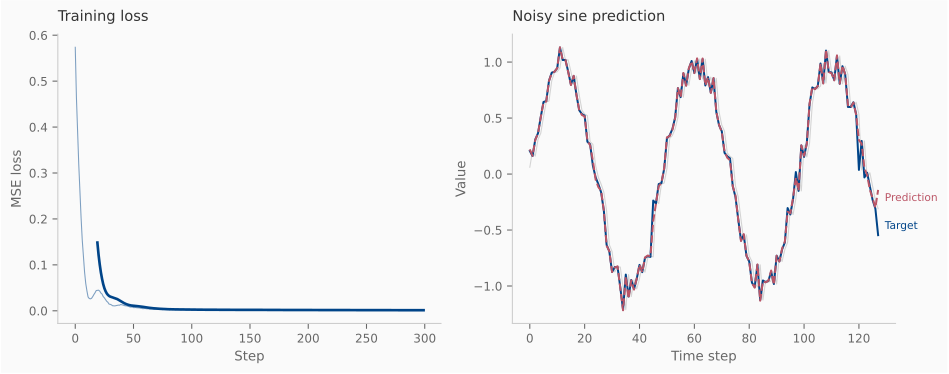
Noisy sine prediction
The synthetic task validates the training harness before plugging in SSM layers. Each sample is a noisy sine wave with random frequency . The target is next-step prediction: .
The reusable make_batch helper returns and appears throughout the curriculum:
| Week | Task | Protocol |
|---|---|---|
| 2 | Noisy sine | make_noisy_sine_batch |
| 7 | Selective copying | make_copy_batch |
| 11 | MQAR | make_mqar_batch |
Layer stacking with nnx.scan
lax.scan (Week 1) | nnx.scan (this chapter) | |
|---|---|---|
| Iterates over | Sequence time steps | Layer depth |
| Carry | State | Hidden activation |
| Body | SSM step function | Residual block |
| Parameters | Same at every step | Different per layer |
The NNX pattern splits initialization from execution:
nnx.vmapover__init__: creates independent parameter sets (one per layer).nnx.scanover__call__: applies the same function sequentially with the carry pattern, using different parameters at each step.
The split_rngs decorator splits the PRNG key so each layer receives a unique random seed for initialization (vmap) or execution (scan):
# Init: vmap creates separate params per layer
@nnx.split_rngs(splits=num_layers)
@nnx.vmap(in_axes=(0,), out_axes=0)
def create_blocks(rngs):
    return ResidualBlock(features, rngs=rngs)

# Forward: scan applies blocks sequentially
@nnx.split_rngs(splits=num_layers)
@nnx.scan(in_axes=(nnx.Carry, 0), out_axes=nnx.Carry)
def forward(h, block):
return block(h)For a stack of residual blocks applied via nnx.scan, each layer Jacobian takes the form rather than just . This often makes gradients easier to propagate through deep stacks, but it does not guarantee nonzero for every layer on every input. Zero loss gradients, saturated activations, or parameter symmetries can still produce zero parameter gradients.
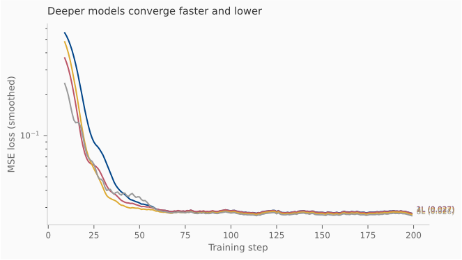
The reusable experiment harness
Custom variable type for SSM parameters
SSM parameters (A, B, ) need different optimizer treatment than backbone parameters (Dense, LayerNorm). The NNX solution: subclass nnx.Variable:
class SSMParam(nnx.Variable):
    """SSM-specific params: low LR, zero weight decay."""
    pass
Then create two optimizers filtered by variable type:
ssm_opt = nnx.Optimizer(model, ssm_tx, wrt=SSMParam)
backbone_opt = nnx.Optimizer(model, backbone_tx, wrt=nnx.Param)
The motivation for two optimizers is that the SSM inner-parameter landscape is narrow — eigenvalues must stay inside a thin band near the stability boundary — while the backbone’s MLP/linear weights tolerate much larger updates. A single learning rate compromises between exploration of the backbone and precision on the SSM; two optimizers let each subspace use its own tempo.
A toy model with and . Both receive unit gradients at every step. With SSM LR and backbone LR (vanilla SGD for clarity), one step moves
Over 1,000 steps travels units while travels — deliberately close in magnitude, with the SSM slightly faster to accelerate eigenvalue search. Pointing a single optimizer at both produces either an SSM that wanders outside the stable cone or a backbone that crawls; separating them resolves the conflict.
Dual optimizer with nnx.DiffState
When computing gradients, we need to tell JAX which parameters to differentiate with respect to. nnx.DiffState(0, SSMParam) means: “in the first function argument (the model), compute gradients only for variables of type SSMParam.” This produces a gradient tree that matches the shape expected by the wrt=SSMParam optimizer.
In Flax 0.12.6, passing full gradients to a wrt-filtered optimizer causes a tree structure mismatch (the optimizer expects only SSMParam leaves, but receives all leaves). The DiffState pattern avoids this:
loss, bb_grads = nnx.value_and_grad(
    loss_fn, argnums=nnx.DiffState(0, nnx.Param)
)(model)
ssm_grads = nnx.grad(
    loss_fn, argnums=nnx.DiffState(0, SSMParam)
)(model)
ssm_opt.update(model, ssm_grads)
backbone_opt.update(model, bb_grads)
SSM training recipe
SSM training requires careful hyperparameter choices. The learning rate (LR) controls how large each gradient update step is. Weight decay is a regularization technique that shrinks parameters toward zero each step, preventing overfitting. SSM parameters (A, B, ) should not have weight decay because their values encode the system dynamics, not learned features. The warmup phase starts training with a very small LR that linearly increases to the peak, avoiding early instability when the model is randomly initialized.
| SSM params | Backbone | |
|---|---|---|
| Optimizer | Adam | AdamW |
| Peak LR | ||
| Weight decay | 0 | 0.01 |
| Schedule | 10% warmup + cosine | 10% warmup + cosine |
| Grad clip | 1.0 global norm | 1.0 global norm |
| Precision | fp32 (required) | fp32 (bf16 optional) |
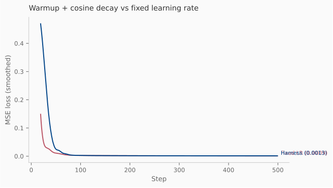
Reflections
Infrastructure investment
This chapter builds plumbing, not research. But every subsequent week plugs into the same harness:
- Week 4: S4 layer replaces
self.convinSimpleSeqModel.SSMParamwraps HiPPO parameters. - Week 6: S5 diagonal SSM uses
lax.associative_scan(Week 1) inside thennx.scan-stacked layers from this chapter. - Week 7: Mamba’s selective scan uses the same dual-optimizer recipe but with input-dependent , , .
- Weeks 11–12: Different synthetic tasks (MQAR, selective copying) follow the
make_batchprotocol. - Week 18: Lyapunov analysis reuses the harness to train SSMs, then analyzes the trained matrices.
What transfers from Week 1
lax.scanhandles SSM time steps, whilennx.scanhandles layer depth. They solve different problems with the same structural pattern.- Automatic differentiation through scans (
jax.grad) works identically for both kinds of scan — the same gradient machinery trains both the SSM parameters and the backbone.