JAX Primitives Through Dynamical Systems
Internalize five JAX primitives — jit, grad, vmap, lax.scan, lax.associative_scan — by implementing dynamical systems you already know: damped oscillator, coupled oscillator ring, EMA. The scan signature (carry, x) → (carry, y) is exactly the SSM state update.
On this page
- Motivation
- The damped oscillator as scan prototype
- Continuous system
- Euler discretization maps to lax.scan
- Energy analysis
- Gradient sensitivity
- fori_loop and jit: alternatives to scan
- Coupled oscillators and the Jacobian
- Ring topology with nearest-neighbor coupling
- Jacobian as transition matrix
- Batching with vmap
- Lyapunov exponents via QR decomposition
- The numerical catastrophe
- The QR algorithm
- Parallel prefix computation
- Warm-up: cumulative sum
- The EMA recurrence
- The associative operator
- Reflections
- What transfers directly from the PhD
- What requires adaptation
- Forward map
Motivation
The standard route into state space models begins with lax.scan tutorials that implement toy counters or fibonacci sequences. We take a different path: implement dynamical systems you have solved before, and let the JAX primitives emerge as the natural computational substrate.
This chapter builds four pieces of infrastructure that recur throughout the curriculum:
- A
lax.scan-based time stepper (used in every SSM implementation), - Automatic Jacobian computation via
jax.jacfwd(stability analysis), - QR-based Lyapunov exponents via
lax.scan(training diagnostics, Week 18), - The associative scan operator for parallel prefix computation (S5, Mamba).
The damped oscillator as scan prototype
Continuous system
Consider the damped harmonic oscillator:
where is the natural frequency and is the damping coefficient. In state-space form with state :
Continuous SSM with (no forcing). Full SSMs add forcing and output .The eigenvalues of are . For underdamped motion (), these are complex with negative real part — the system oscillates and decays. This eigenvalue structure is identical to what we will see in trained S4D layers (Week 5).
Euler discretization maps to lax.scan
Forward Euler with step size :
This is a recurrence of the form — exactly the pattern that lax.scan computes. The scan signature (carry, x) -> (carry, y) maps as:
| Scan element | SSM role | Oscillator |
|---|---|---|
carry | state | |
x | input | (unused — autonomous system) |
y | output |
With , , , and initial , one Euler step gives
The position has not moved yet; velocity has picked up the restoring force. This is the pair that carry = (x, v) stores and hands to the next step — lax.scan automates exactly this handoff over the full trajectory.
The lax.scan implementation and the Python for-loop implementation of the damped oscillator compute the same recurrence and therefore agree up to floating-point roundoff under the current implementation.
Both compute the same recurrence with the same initial condition. lax.scan is a compiled version of the sequential loop — it does not reorder or fuse operations across time steps. The only difference is compilation: lax.scan traces the step function once and executes the compiled XLA loop, while the Python loop re-interprets each step. In practice the trajectories match to machine precision because the same floating-point operations are applied in the same sequence.
Energy analysis
The energy satisfies . For , energy decays monotonically in continuous time.
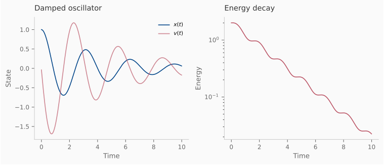
Gradient sensitivity
JAX’s jax.grad computes — the sensitivity of the endpoint to the damping coefficient. This works through the entire lax.scan via reverse-mode automatic differentiation.
The ability to differentiate through a scan is what makes SSMs trainable. When we add learnable parameters (, , , ), the same jax.grad machinery computes gradients for all of them simultaneously.
fori_loop and jit: alternatives to scan
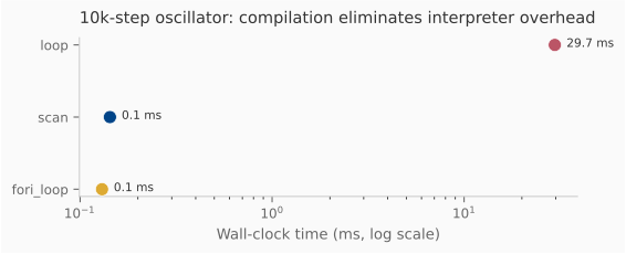
lax.fori_loop compiles the same recurrence but returns only the final state — no trajectory stored. This is the inference pattern: when generating tokens, you need , not the intermediate .
jax.jit wraps the entire scan into a single XLA computation, eliminating Python interpreter overhead between steps. The first call traces and compiles; subsequent calls dispatch directly to the compiled kernel.
lax.scan and fori_loop run 10–100× faster than the Python loop.
[Convergence]
Coupled oscillators and the Jacobian
Ring topology with nearest-neighbor coupling
oscillators on a ring, coupled via discrete Laplacian:
The state vector is .
Jacobian as transition matrix
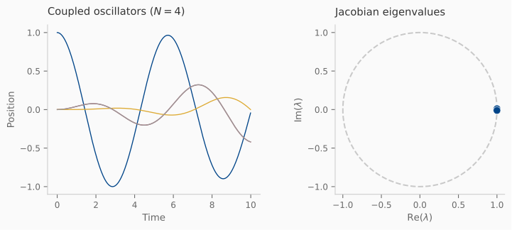
The Jacobian of one Euler step with respect to the state, , is the matrix of all first-order partial derivatives — it captures how a small perturbation in propagates through one time step. This makes the discrete-time transition matrix: it describes how the state evolves locally.
For linear systems, is constant (independent of ) — the same transition applies everywhere. For nonlinear systems, varies along the trajectory. In the SSM context, this distinction maps to Linear Time-Invariant (LTI) models (S4, S4D) where parameters are fixed, versus selective models (Mamba) where parameters depend on the input. ”Selective” means the model can choose what to remember based on input content, not just position.
We compute via jax.jacfwd(one_step)(state0), which returns the full Jacobian matrix.
Batching with vmap
jax.vmap vectorizes a function over a batch dimension without writing explicit loops. It transforms a function into that processes inputs simultaneously on GPU.
Two demonstrations:
- Ensemble simulation:
vmapover initial conditions produces oscillator trajectories in parallel. This is the same pattern used to process a minibatch of sequences through an SSM layer. - Batched Jacobians:
vmap(jacfwd)computes the transition matrix at different states simultaneously. In Week 18, this enables Lyapunov analysis across minibatches of sequences.
vmap composes with other JAX transforms. Applied to grad, it yields per-example gradients; wrapped in jit, it compiles the batched computation. This composability is why JAX fits SSM research so well: scan, vmap, and grad combine in the same pattern you would write mathematically.
Lyapunov exponents via QR decomposition
Executable companion:guides/notebooks/week01_notebook.ipynb Exercise 3 computes the full spectrum with the QR pattern described here.
The numerical catastrophe
Given a sequence of transition matrices , the cumulative effect is the product . Computing directly is numerically catastrophic: if any eigenvalue has , components grow exponentially (), causing overflow. If , components decay to zero (underflow). With steps, even grows to .
The QR algorithm
Due to Benettin et al. (1980) . Oseledets’ theorem guarantees convergence: the time-averaged growth rates exist and are independent of the initial perturbation directions almost everywhere.The solution is to periodically orthogonalize via QR decomposition. [Official] Benettin et al. Benettin et al. (1980) introduced the algorithm; see Anonymous (2025) for a recent application in the SSM context. At each step:
- Propagate the perturbation matrix:
- Decompose: (QR factorization)
- Accumulate:
The Lyapunov exponents are the time-averaged growth rates:
The computation fits naturally into lax.scan. Its carry stores the state, the orthogonal basis, and the running log sum:
This is the same carry-and-update pattern used by SSM recurrences.
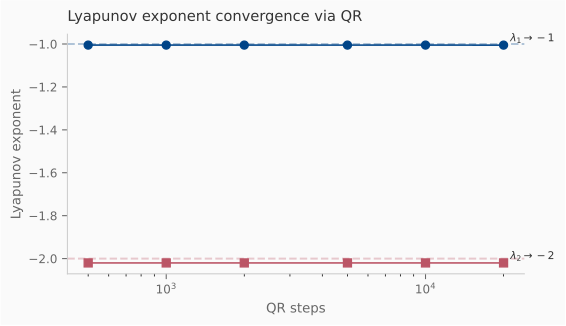
For the linear system with , the Lyapunov exponents computed from the Euler-step Jacobian satisfy
In the continuous-time limit , this converges to .
For a diagonal system, the Jacobian of the Euler step is . The QR decomposition is trivial (, ), so
Expanding shows as . With and 10,000 steps, the error is in our experiments.
For the same Euler-discretized linear system,
Consequently, as .
Summing the previous formula gives
Since the eigenvalues of are , the product is . Taking recovers from the standard expansion .
Parallel prefix computation
Warm-up: cumulative sum
The simplest associative_scan example: cumulative sum with the operator . Addition is trivially associative, so:
def cumsum_associative(x):
    return jax.lax.associative_scan(jnp.add, x)
This produces identical results to jnp.cumsum but makes the parallel prefix structure explicit. The Blelloch algorithm Blelloch (1990)
computes all prefix sums in parallel depth — a general technique for reducing an associative operator over a sequence in parallel steps using total work. Same FLOPs as a sequential scan, but vastly more parallelism on GPU.
The EMA recurrence
The exponential moving average (EMA) is a running weighted average that gives more weight to recent values. With smoothing parameter :
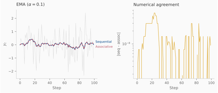
When is small (e.g., 0.1), the average is “slow” and remembers far into the past. When is large (e.g., 0.9), it tracks the input closely. This is a first-order linear recurrence — the simplest possible SSM with scalar state, , and .
Sequential computation via lax.scan requires sequential steps. Can we do better?
The associative operator
Define the pair representation , where is the decay factor and is the input contribution. We need a binary operator — a function that combines two such pairs into one, representing the combined effect of two consecutive time steps. The key requirement is associativity: , which allows arbitrary grouping and therefore parallel evaluation. The operator:
The scan operator is associative.
Compute both groupings:
Both expressions are identical.
Associativity is what enables jax.lax.associative_scan to compute the prefix sums in parallel depth using Blelloch’s algorithm.
Reflections
What transfers directly from the PhD
Three pieces of infrastructure from vortex dynamics research reappear with zero modification:
- QR-based Lyapunov computation. Same algorithm, same numerical considerations (transient removal, convergence diagnostics). The only adaptation: SSM dynamics are input-dependent, so the spectrum is a statistic over sequences rather than a property of the system.
- Discretization awareness. The intuition that “choice of integrator determines long-time accuracy” maps directly to “choice of SSM discretization determines training stability.” The stability region analysis from numerical methods applies unchanged.
- Eigenvalue monitoring. Tracking whether eigenvalues stay in the left half-plane (continuous) or inside the unit disk (discrete) is the same diagnostic in both domains.
What requires adaptation
- No natural period. Floquet theory assumes periodicity; SSM dynamics depend on the input sequence. The correct analogue is Lyapunov exponents (infinite-time average) rather than Floquet multipliers (one-period product).
- High dimension. The vortex quartet has 4–8 degrees of freedom. SSMs have – per layer, with – time steps. The QR algorithm scales well (), but visualization strategies change.
- Learned dynamics. In the dissertation, is given by physics. In SSMs, is learned — meaning the stability properties change during training. This opens the question of whether stability-aware training (constraining eigenvalues) improves optimization.
Forward map
- Week 2: The training loop harness built in Flax will use
lax.scanfor the SSM layer andoptaxfor optimization. - Weeks 4–6: S4, S4D, and S5 use the exact scan patterns from this chapter, with HiPPO-initialized matrices instead of our hand-crafted oscillator systems.
- Week 7: Mamba makes , , and input-dependent, breaking the convolutional view but preserving the parallel scan.
- Week 18: The Lyapunov infrastructure from Exercise 3 is applied to trained SSMs to characterize gradient flow stability.
- Week 20: The discretization analysis from the DynConnect boxes is formalized with stability region plots in Julia.