Part II · SSM Core Week 5 Published s4d.py test_s4d.py Notebook

Diagonal SSMs (S4D) and Stability Analysis

S4D — the diagonal simplification of S4 that drops kernel cost from O(N²L) to O(NL) and makes stability guaranteed by construction via log-parameterized eigenvalues.

On this page

From Full to Diagonal
Initialization variants
S4D-Lin (default)
S4D-Inv
S4D-LegS
Complex-valued state and stability by construction
Element-wise computation
Stability region analysis
Reflections
What transfers
What requires adaptation
Forward map

From Full to Diagonal

Week 4’s S4 stores $\statemat$ as a full $\statedim \times \statedim$ matrix (HiPPO-LegS initialization). The kernel computation $K[k] = \outputmat \discA^k \inputmat$ requires matrix powers — $\bigO{\statedim^2\seqlen}$ even with a naive implementation.

S4D’s insight: any diagonalizable SSM with distinct eigenvalues can be transformed to an equivalent diagonal form. “Diagonal” here means the state matrix $\statemat$ is a diagonal matrix (all off-diagonal entries zero), not a reference to any architectural name. The key result comes from the DSS (Diagonal State Space) paper Gupta et al. (2022) : the change-of-basis $V$ that diagonalizes $\statemat$ via eigendecomposition can be absorbed into $\inputmat$ and $\outputmat$ without changing the system’s input-output behavior.

Proposition 5.1 (Diagonal expressiveness).

If $\statemat = V \Lambda V^{-1}$ with distinct eigenvalues $\Lambda = \diag(\lambda_1, \ldots, \lambda_\statedim)$ , then the SSM $(\statemat, \inputmat, \outputmat)$ has the same transfer function as $(\Lambda, V^{-1}\inputmat, \outputmat V)$ . The transfer function $G(z) = \outputmat(zI - \statemat)^{-1}\inputmat$ captures the complete input–output behavior of the system — two SSMs with the same transfer function produce identical outputs for any input.

Proof.

The transfer function is $G(z) = \outputmat(zI - \statemat)^{-1}\inputmat$ . Substituting $\statemat = V\Lambda V^{-1}$ : $G(z) = \outputmat V(zI - \Lambda)^{-1}V^{-1}\inputmat = \tilde{\outputmat}(zI - \Lambda)^{-1}\tilde{\inputmat}$ where $\tilde{\outputmat} = \outputmat V$ and $\tilde{\inputmat} = V^{-1}\inputmat$ .

Initialization variants

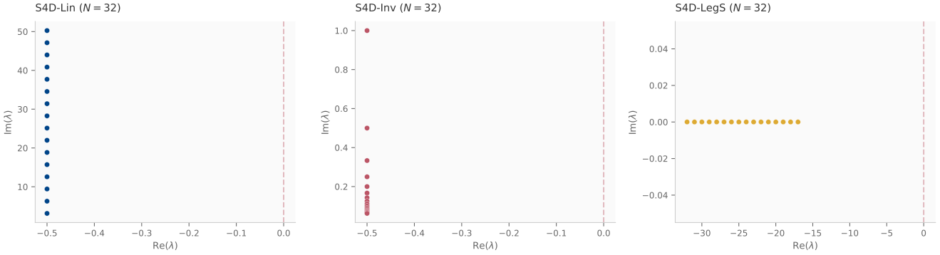
S4D stores eigenvalues as complex numbers: $\lambda_k = a_k + i \cdot b_k$ where $a_k < 0$ (decay) and $b_k$ (oscillation frequency). Three initialization schemes:

S4D-Lin (default)

$\lambda_k = -\tfrac{1}{2} + i \pi k$ for $k = 1, \ldots, \statedim/2$ . [Convergence] S4D-Lin is the default initialization in the S4D, S5, and mamba-minimal reference codebases; other schemes are empirical variants.

Constant decay rate $-1/2$ , linearly spaced frequencies. The simplest formula — one line of code. Each eigenvalue captures a different frequency band of the input signal. S4D-Lin is not the best performer on long-range tasks, but its simplicity makes it ideal for understanding the diagonal structure.

Example 5.2 (S4D-Lin at N = 8).

Four complex-conjugate pairs $\{-0.5 + i k\pi : k = 1, 2, 3, 4\}$ . All share decay rate $-0.5$ but span frequencies $\pi$ through $4\pi$ . With $\stepsize = 0.1$ ,

\abs{\bar\lambda_k} = \abs{\exp(\lambda_k\stepsize)} = e^{-0.05} \approx 0.951 \quad \text{(same for every } k\text{)},

so every channel’s state decays by ~5% per step. The phase rotation is $\angle\bar\lambda_k = 0.1\pi k$ radians per step: $0.1\pi$ , $0.2\pi$ , $0.3\pi$ , $0.4\pi$ . Each channel acts as a bandpass filter centered on its frequency, and their sum reconstructs any bandlimited signal the eight-dimensional basis can resolve.

S4D-Inv

$\lambda_k = -\tfrac{1}{2} + i/k$ for $k = 1, \ldots, \statedim/2$ .

Inverse frequency spacing concentrates resolution at low frequencies, which is better for long-range dependencies.

S4D-LegS

Extract the diagonal of the HiPPO-LegS eigendecomposition from Week 4: compute $\operatorname{eigvals}(\statemat_{\text{HiPPO}})$ and use the $\statedim/2$ eigenvalues with most negative imaginary part.

Eigenvalue patterns for the three S4D initialization variants. S4D-Lin: uniformly spaced frequencies with constant decay. S4D-Inv: inverse frequency spacing concentrating resolution at low frequencies. S4D-LegS: eigenvalues extracted from HiPPO decomposition (approximately real).

Complex-valued state and stability by construction

S4D uses $\statedim/2$ complex eigenvalue conjugate pairs. A conjugate pair means: if $\lambda_k = a + bi$ is an eigenvalue, then $\lambda_k^* = a - bi$ is also an eigenvalue (same real part, negated imaginary part). We only need to store one of each pair and reconstruct the other. This halves the parameter count and, crucially, guarantees real-valued output through the identity $z + z^* = 2\operatorname{Re}(z)$ . The output uses this conjugate symmetry trick:

y_t = 2 \cdot \operatorname{Re}\!\left(\sum_{k=1}^{\statedim/2} \outputmat_k \cdot \statevec_{k,t}\right) + \feedmat \cdot u_t.

Proposition 5.3 (Stability by construction).

With the parameterization $\operatorname{Re}(\lambda_k) = -\exp(\texttt{log\_w\_real}_k)$ and $\operatorname{Im}(\lambda_k) = \texttt{w\_imag}_k$ , all continuous eigenvalues satisfy $\operatorname{Re}(\lambda_k) < 0$ for any finite parameter values. ZOH discretization then maps these inside the unit disk: $\abs{\bar{\lambda}_k} = e^{\operatorname{Re}(\lambda_k) \cdot \stepsize} < 1$ .

Proof.

$-\exp(x) < 0$ for all $x \in \R$ . The ZOH stability preservation follows from [?w4:prop:zoh-stability].

This is a crucial difference from Week 4: S4’s HiPPO initialization happens to be stable, but training could push eigenvalues out of the left half-plane. S4D’s log-parameterization makes continuous eigenvalue instability impossible by construction under this parameterization. [Official] The log-parameterization $\Re(\lambda_k) = -\exp(\texttt{log\_w\_real}_k)$ originates in the S4D paper Gu et al. (2022) and reproduces across S5, Mamba-1, and Mamba-2 reference code. Finite-precision accumulation, gradient overflow, and extreme- $\stepsize$ artifacts are still possible; stability-by-construction fixes only the sign of $\operatorname{Re}(\lambda_k)$ .

Element-wise computation

With diagonal $\statemat$ , all matrix operations collapse to element-wise:

Proposition 5.4 (Kernel complexity reduction).

For diagonal $\discA = \diag(\bar{\lambda}_1, \ldots, \bar{\lambda}_{\statedim/2})$ , the convolution kernel is:

K[\ell] = 2 \cdot \operatorname{Re}\!\left(\sum_{k=1}^{\statedim/2} \tilde{\outputmat}_k \cdot e^{\lambda_k \stepsize \cdot \ell}\right),

where $\tilde{\outputmat}_k = \outputmat_k \inputmat_k \cdot \frac{e^{\lambda_k \stepsize} - 1}{\lambda_k}$ absorbs the ZOH correction. This is $\bigO{\statedim \seqlen}$ vs. $\bigO{\statedim^2 \seqlen}$ for full $\statemat$ .

Proof.

Since $\discA$ is diagonal, $\discA^k = \diag(\bar{\lambda}_1^k, \ldots)$ . The matrix product $\outputmat \discA^k \inputmat$ decomposes into $\statedim/2$ independent scalar products. The log-space computation $e^{\lambda_k \stepsize \cdot \ell}$ avoids explicit power iteration.

The recurrence also simplifies:

\statevec_{k,t+1} = \bar{\lambda}_k \cdot \statevec_{k,t} + \tilde{\inputmat}_k \cdot u_t \qquad \text{(element-wise, not matrix multiply)}.

def ssm_recurrent_diag(Ab_diag, B, C, D, u):
    def step(h, u_t):
        h_new = Ab_diag * h + B * u_t     # element-wise
        y_t = 2 * jnp.real(jnp.sum(C * h_new)) + D * u_t
        return h_new, y_t
    h0 = jnp.zeros_like(Ab_diag)
    _, y = jax.lax.scan(step, h0, u)
    return y

Numerical trace: diagonal recurrence

Consider a 2-state diagonal SSM with eigenvalues $\lambda_1 = -0.5 + 3i$ , $\lambda_2 = -0.5 - 3i$ (conjugate pair), step size $\stepsize = 0.1$ , and input $u = [1, 0, 0, \ldots]$ (unit impulse).

Discretize: $\bar{\lambda}_k = e^{\lambda_k \stepsize}$ , so $\bar{\lambda}_1 = e^{(-0.05 + 0.3i)} = e^{-0.05}(\cos 0.3 + i\sin 0.3) \approx 0.907 + 0.281i$ .

Step 0: $\statevec_0 = [0, 0]$ .

Step 1: $\statevec_{1,k} = \bar{\lambda}_k \cdot 0 + \tilde{B}_k \cdot 1 = \tilde{B}_k$ . Each state component is an independent scalar multiply — no matrix product needed.

Step 2: $\statevec_{2,k} = \bar{\lambda}_k \cdot \statevec_{1,k} + \tilde{B}_k \cdot 0 = \bar{\lambda}_k \tilde{B}_k$ . The magnitude decays: $\abs{\bar{\lambda}_1}^2 \approx 0.905^2 \approx 0.819$ . The phase rotates: the state oscillates while shrinking.

Output: $y_t = 2\operatorname{Re}(\outputmat_1 \statevec_{1,t} + \outputmat_2 \statevec_{2,t})$ — the conjugate symmetry cancels imaginary parts, giving real output.

Compare with full S4: the same computation requires $\discA^2 \inputmat$ (matrix–matrix–vector products). Diagonal S4D reduces this to element-wise scalar operations.

Stability region analysis

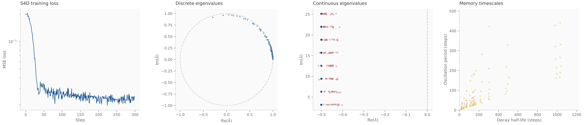
The [DYN] exercise: compare learned eigenvalue positions against integrator stability boundaries.

Integrator stability regions meet SSM eigenvalues

Every discretization method (Euler, ZOH, bilinear) maps a region of the continuous complex plane $\lambda\stepsize$ to the unit disk. The S4D eigenvalues, after training, should cluster inside the intersection of:

The left half-plane (continuous stability)
The ZOH stability region (always the full left half-plane)
The learned step size’s “sweet spot” (where $\abs{e^{\lambda\stepsize}}$ is neither too close to 0 nor too close to 1)

The phase portrait (here used in the SSM sense, not the ODE phase-plane sense) maps each eigenvalue’s position in the complex plane to its physical effect on the model’s memory. Specifically: magnitude $\abs{\bar{\lambda}_k}$ controls the decay half-life $t_{1/2} = -\log 2 / \log\abs{\bar{\lambda}_k}$ (how many time steps until the state’s influence decays by half), and phase $\angle\bar{\lambda}_k$ controls the oscillation period $T = 2\pi / \abs{\angle\bar{\lambda}_k}$ .

This is the same stability–accuracy trade-off you analyzed in your PhD for Floquet multipliers of periodic orbits — now applied to learned neural network parameters.

S4D training dynamics and stability analysis. Top-left: training loss (log scale). Top-right: discrete eigenvalues inside the unit disk (pre- and post-training). Bottom-left: continuous eigenvalues in the left half-plane. Bottom-right: phase portrait mapping eigenvalue position to decay half-life and oscillation period.

Reflections

What transfers

Diagonal = element-wise: The single most impactful simplification in the S4 lineage. Every subsequent architecture (S5, Mamba) uses diagonal state.
Stability by construction: The log-parameterization eliminates a class of training failures. This pattern reappears in LRU Orvieto et al. (2023) and Mamba.
Phase portrait analysis: Eigenvalue position → memory timescale is the key diagnostic for understanding what an SSM has learned.

What requires adaptation

Complex arithmetic overhead. The conjugate-pair trick halves parameters but introduces complex-valued computation throughout the forward pass. JAX handles complex64 natively, but a common failure mode is dtype mismatch: a function expecting float32 receiving complex64 (or vice versa) produces silent wrong results or cryptic shape errors. Always check dtypes at module boundaries.
Loss of the HiPPO interpretation. Full S4’s state vector has a clean theoretical meaning: each entry is a Legendre coefficient of the input history. Going diagonal discards this — the state becomes a collection of independently decaying oscillators with no polynomial approximation guarantee. This is an explicit theory-for-speed trade-off: the output is empirically similar, but the interpretability of the state is lost. S4D-LegS partially recovers the connection by initializing from HiPPO eigenvalues, but training immediately drifts away from the Legendre structure.
Initialization choice becomes empirical. Unlike Week 4’s HiPPO (one principled answer derived from approximation theory), S4D offers three variants with different frequency-resolution trade-offs: S4D-Lin (uniform resolution), S4D-Inv (low-frequency emphasis), and S4D-LegS (HiPPO-derived). [Practitioner] Choosing between them requires benchmarking on your target task — there is no single “correct” initialization. This is the first point in the curriculum where design becomes empirical rather than principled.

Forward map

Week 6: S5 replaces lax.scan with associative scan for $\bigO{\log \seqlen}$ parallel depth. The diagonal structure from this week is required.
Week 7: Mamba makes $\inputmat, \outputmat, \stepsize$ input-dependent, breaking the convolutional view. The diagonal state and log-parameterization carry over.
Week 18: Lyapunov analysis of the eigenvalue dynamics during training — tracking how the learned eigenvalues drift over optimization steps.